Anomaly Detection at 40 MHz
Introduction
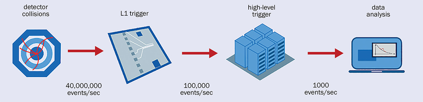
The Compact Muon Solenoid (CMS) Experiment at CERN produces massive amounts of data every second ($ \sim \mathcal{O}(40)$ TB/s), most of which is not practically stored or even analyzedanalyzed entirely. To solve this issue, several filtration steps or triggers have been developed that operate hierarchically to filter the amount of incoming data and reduce the number of events (collision events) from 40 MHz to a manageable 1 kHz. Two triggering steps achieve this:
- Level 1 Trigger (L1T): This is the first trigger that operates mainly on Field Programmable Gate Array (FPGAs) and is responsible for reducing the rate from 40 MHz to 100 kHz.
- High Level Trigger (HLT): This is the second trigger that operates on CPU and GPU farms and uses a complete physics analysis (reconstruction) to make the trigger decision. HLT reduces the data rate from 100 kHz to 1 kHz.
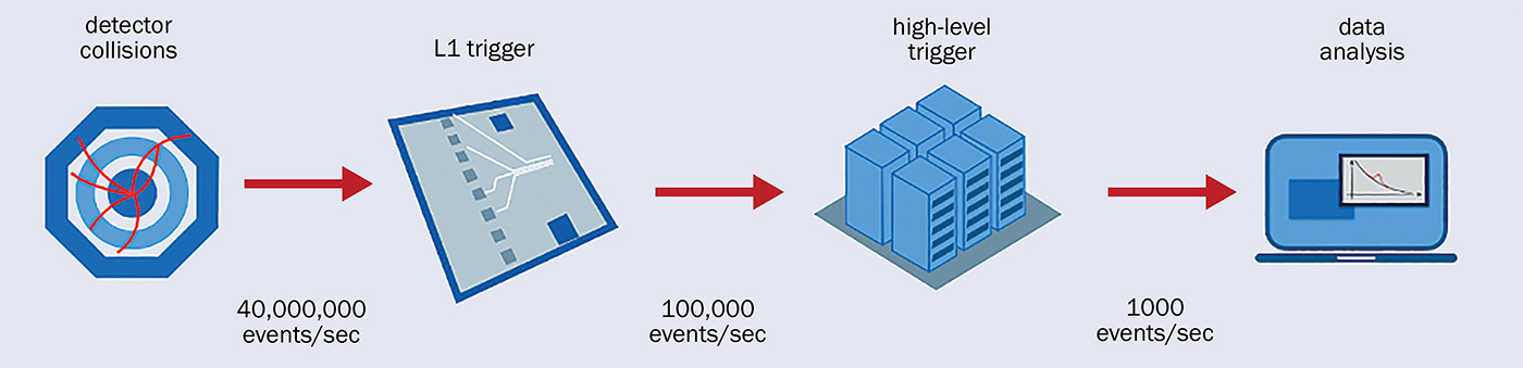
Given the massive amount of data, a rough resolution (portion of the entire data) of the events is used to make a decision for the L1T, making physics reconstruction algorithms impossible. Hence, L1T is primarily a cut-based trigger, where thresholds for physics observables are set as criteria for trigger conditions. Even though L1T works exceptionally well and has been heavily developed and tuned for quite some time, it remains heavily biased by the physical intuitions and assumptions used to build it.
The Standard Model (SM) of physics, being one of the most successful theories in modern physics, still fails to account for several phenomena, such as the existence of gravity as a distinct entity from the other fundamental forces, CP Violation, and the existence of dark matter, among others. All these discrepancies have led to theories that try to incorporate these phenomena. For the verification of such theoretical Beyond Standard Model (BSM), the discovery of new BSM particles is necessary. Given that BSM is an uncharted territory that might or might not follow the physical assumptions of the existing L1 Trigger, calls for the development of a new, unbiased trigger, completely from scratch, that can efficiently filter data and remain based entirely on statistical properties rather than physics-based intuitions.
AXOL1TL
Anomaly eXtraction Online L1 Trigger Lightweight in L1 Global Trigger (AXOL1TL) is a trigger based on an anomaly detection algorithm that is deployed as a part of the L1T, which takes in a subset of the Level-1 (L1) objects (measurables) and tries to assign an anomaly score for every event. Events are selected based on their anomaly score, considering fixed-rate budgets.
Working of the existing baseline
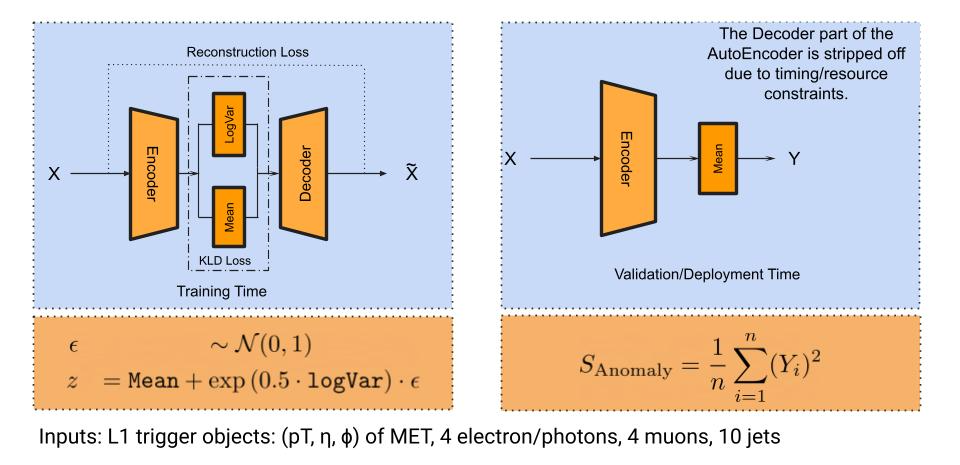
The diagram above illustrates the training and deployment of the baseline (v4) model. In this report, we discuss how we can improve on this architecture to make the trigger more accurate (in detection), robust (to changing detector conditions), and interpretable (for analysis).
The above method exhibits a few problems:
- The loss (used to train) the original Variational AutoEncoder (VAE) for anomaly detection (AD) does not align well with the final optimisation goal of the model, given that the headless (without Decoder) model no longer represents an autoencoder. Using latent vectors (in this case, their L2 norm) for anomaly detection can be challenging and unpredictable.
- VAEs do not guarantee any form of explicit clustering in the embedding space where similar samples strictly lie close to each other. Reconstruction error of a point might hint toward it being anomalous, but the same is not always valid for points that are close to each other (or have similar L2 norm).
- Taking the L2 norm of the latents explicitly assumes that the anomalous samples will always be strictly away from the center, but that might not always be true.
To address these problems, we modify the VAE. The modification will be discussed and developed over the course of the following few sections.
Self-Supervised Learning, metric and clustering.
Self-Supervised Learning (SSL) is a ML paradigm that focuses on the production of information-rich feature vectors from a dataset without explicitly using any labels. To achieve this, SSL models are trained on a surrogate task that utilizes pseudo labels from training and loss computation. For this study, we primarily focus on the VICReg, a well-celebrated SSL technique.
VICReg
VICReg: Variance-Invariance-Covariance Regularization for Self-Supervised Learning work by training on the surrogate task of generating embedding spaces that are invariant to specific augmentation spaces. This is achieved by using a Siamese-like setup, where two views of the same event are used, but both have been augmented to different degrees. The Euclidean distance in the embedding space between these two views is then minimised using gradient descent.
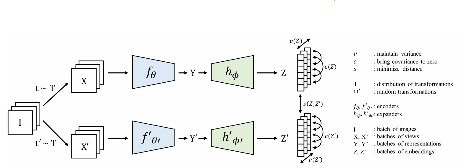
Along with the MSE loss that acts across the two projection vectors Z, to ensure stability against collapse and the non-triviality of the embedding space, we have covariance and variance regularization terms. The covariance component prevents the embedding dimensions from capturing the same information. In contrast, the variance component prevents all embedding vectors in a batch from collapsing to a single point in the representation space.
Metric
When working with latent spaces, we are often interested in defining a metric on them. The definition of metric or distance in the embedding space provides insight into the exact nature of the embedding space. The metric on the latent space of an autoencoder is often ill-defined due to its erratic nature. Even though VAEs have partially solved this problem by making the space continuous through variational sampling, where two similar samples have similar embeddings due to the variational step, which facilitates the definition of local structures, the metric definition on a global level remains ill-defined. VICReg addresses this by introducing augmentations that often introduce inductive biases within the system, making the global structures clearer.
To get a stronger intuition of this idea, we will take a real-life example. We consider a cylindrical system ($r\cos{t}$,$r\sin{t}$,$h$) where the rotation across the axis (of the cylinder) is invariant to our use cases. We can think of it as a coordinate change. We fix the radius to 1 and the dimension of the embedding space to 2 for easier visualization. The input dataset looks like
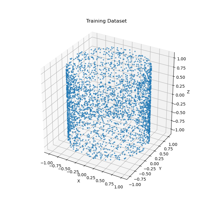
When we train a VAE and a VICReg encoder (with the same architecture) on this dataset, we observe the following latent space.
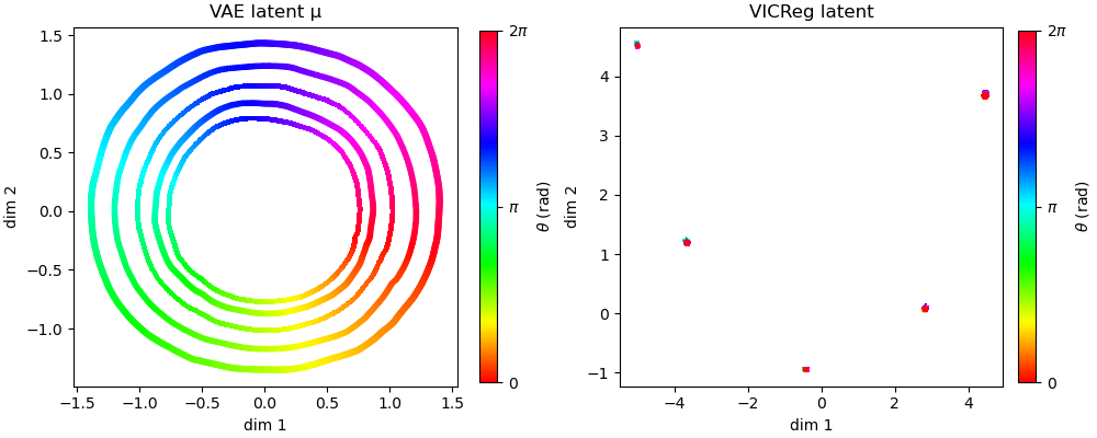
As is already evident, VICReg does a fantastic job of removing the angular component from within the data. We can use the MSE distance between the points in this case for our theta invariant task. The same is not true for VAE; as it is an information-preserving system, it cannot eliminate the angular component, making the concept of distance in our latent space ambiguous. One thing to exercise caution in this entire argument is that the distance is only relevant with respect to proper augmentations. With only Gaussian blurring, we won't be able to define a metric even with our VICReg setup. Removing the rotation from the augmentation space renders our metric for VICReg's latent space ill-defined for our task at hand, where rotation along the axis does not alter the system. Below, we illustrate the nature of the latent space of VICReg without rotation augmentation.
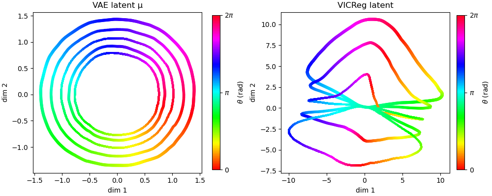
Using different augmentation strategies, we can easily encode various types of invariances within our system, making VICReg an ideal choice to build an embedding space. The metric in this space is the Euclidean distance between two points, indicating how the two separate events differ from each other. Moreover, within each cluster of points in the VICReg space, we can expect samples that are physically invariant to one another (i.e., samples that have different representations in $R^n$ but have similar physical meanings, such as Lorentz-boosted samples or rotated samples). Building systems that can cluster our anomalous samples together is our first step in developing our unified anomaly detection framework.
Anomaly Detection, Density and Clusters
VAEs are one of the best candidate models for anomaly detection (AD). VAEs work well in AD since they fail to reconstruct points that lie in low-density regions, which the model has difficulty learning. The figure below illustrates the operation of a VAE in the context of anomaly detection, when trained on a dataset of 5 overlapping Gaussians in a 2D space.
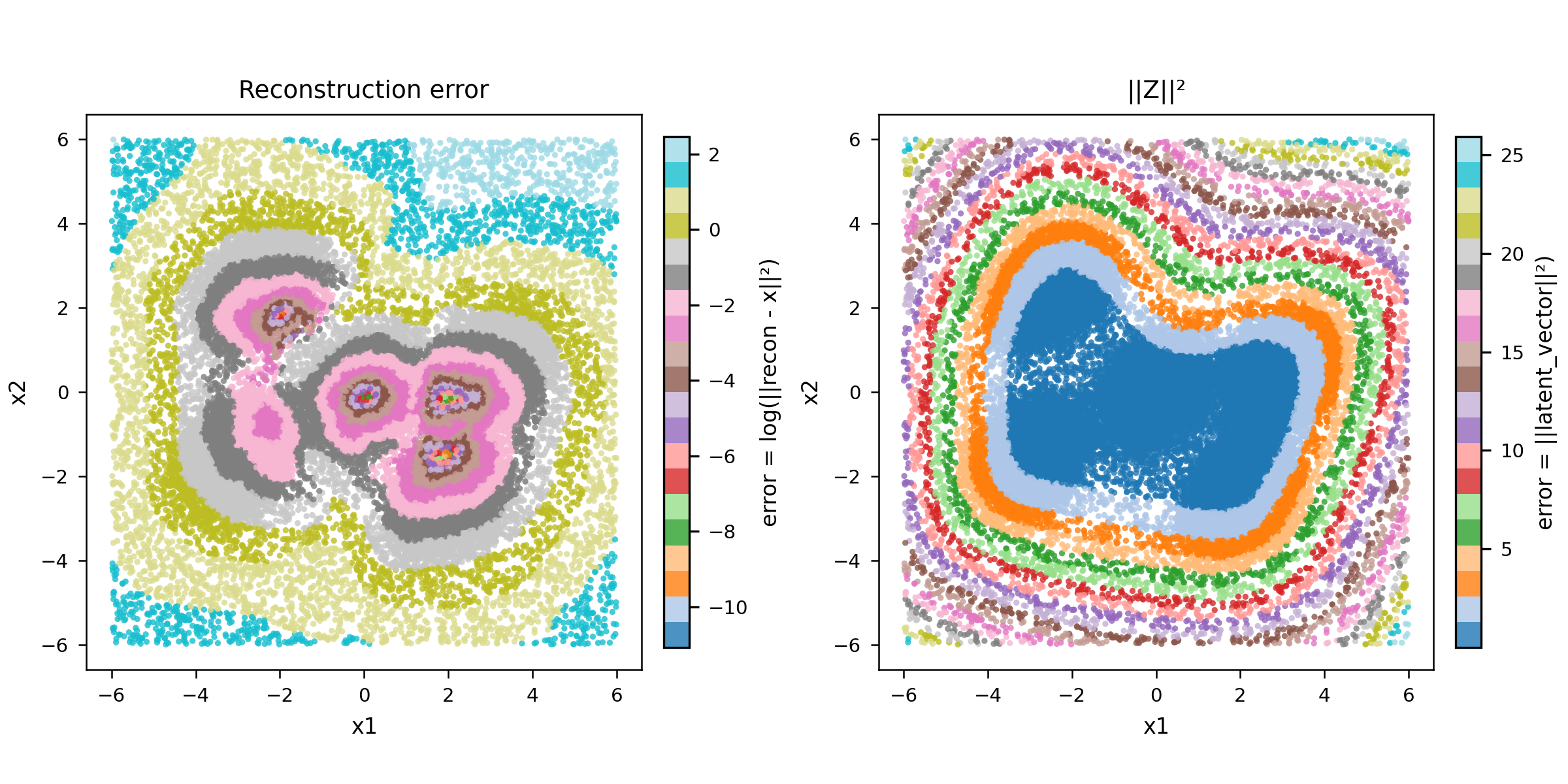
As we can see, when using the standard reconstruction loss, we can correctly identify the 5 cluster centers along with their distribution. In contrast, the surrounding region has a higher reconstruction loss, as there are fewer pointers available there. Although the $||z||_2$ (on the right) or $\mathbf{z}^\top \mathbf{z}$ setup without the Decoder (following the v4 architecture of AXOL1TL) works well in the vicinity of the cluster and in finding the global region of high density, but fails to capture the details of the distributions.
Out-of-the-box-distribution VAEs, as demonstrated, can have good anomaly detection capacities until they encounter the Out-of-the-box-distribution problem, in which case the VAE learns too well about the dataset and ends up reconstructing everything (including the anomalies) perfectly, making it a poor choice for anomaly detection in those cases. This problem can get further aggravated when the training dataset itself contains the anomalous datapoints (true in our case).
On the other hand, although we have established the paradigm of latent space creation through VICReg and formed tight clusters of points, we have yet to address the problem of identifying clusters where our anomalies or rare samples reside.
Mahalanobis Distance, Gaussian Mixtures and Anomaly Detection
Self-supervised methods, such as VICReg, due to their inherent nature of minimizing invariance loss over the embedding space, tend to create clusters in the latent embedding space. We can broadly classify the entire dataset D to be composed of three components:
- Clusters of Normals (Inliers): By normalies, we understand the physics processes/signals that occur frequently and can be readily found using the existing physics-based triggers. These inliers are defined based on their statistical significance, and such clusters are considered to have a large number of elements and strong distribution peaks. These clusters are importantimportant for Standard Model studies,, but given that we are here trying to look for exotic signatures that are statistically outnumbered,, we refer to these standard physics processes as our normals. We are not particularly interested in probing these clusters in this work, given the extensive amount of research that has already been conducted on such processes. Let's denote them by the notation $N_i$, we can have many such physics processes, all of which can be categorised into their own clusters as $N_0, N_1...N_n$
- Cluster of Anomalies: Given the pretext that the anomalies follow a different form of distribution pattern within the dataset, given that they originate from exotic physics processes, we can consider these anomalies to be contained within their own clusters, just like the nomalies, except these cluster centers are separated from $N_i$. Given that we assume these anomalies are indicative of exotic physics signatures, they must be present in clusters. The absence of clusters for anomalies means they can never be detected with certainty using our framework, which points towards a deeper problem, such as poor detector resolution or a poor choice of augmentation/architecture. Lets call these $A_0,..A_1,...A_a$
- Stray points: For the sake of completion, we can consider the remaining points to be spread across the embedding space. These points are generally statistical noise and can be attributed to various sources, including hadronic noise and detector issues. We can refer to all these points $S_0, S_1... S_s$
Given that there does not exist a rigid definition distinguishing $S$ and $A$, and that in the absence of a well-defined embedding space or identifiable anomalies, $S$ may consist of shallow distributions or even isolated points—which are inherently difficult to model—we absorb all $S$ into $A$.
We can now say $D = \left( \bigcup_{i \in n} N_i \right) \times \left( \bigcup_{j \in J} A_j \right)$
Now, finding $\bigcup_{i \in I} N_i$ is straightforward, as these correspond to some of the most well-studied processes in high-energy physics (HEP). However, we deliberately refrain from invoking physical intuition, as our goal is to construct an unbiased system. Instead, we adopt the statistical definition of $N_i$ — treating them as the most well-populated distributions.
We take a hyper-parameter $k \in \mathrm{N}$ assuming that we have $K$ clusters of normals. Now we fit a Gaussian mixture model (GMM) on the latent space with $k$ gaussians, making sure that all our standard physics signatures get absorbed within these $k$ clusters. Now, for any point $p$ on the embedding space, we can find how anomalous it is by finding how far it is from these cluster centers.
Had the value of $k$ been 1. We could have used the Mahalanobis distance for finding the distance of $p$ from the cluster center. For finding the distance of a point $p$ from $k$ gaussians, one can use methods like these. Given that such methods are extremely difficult to implement on an FPGA board (where we want to deploy our model), we skip it. Instead, we try to compute $D_i$ for $p$, where we define $D_i$ using the mahalanobis distance as
where:
- $\mathbf{p}$ — point or event in the embedding space whose anomaly score is being evaluated.
- $D_i(\mathbf{p})$ — Mahalanobis distance of point $\mathbf{p}$ from the $i^{\text{th}}$ cluster center.
- $\boldsymbol{\mu_i}$ — mean of the $i^{\text{th}}$ cluster in the embedding space.
- $\mathbf{\Sigma_i}$ — covariance matrix of the $i^{\text{th}}$ gaussian on the embedding space.
Now, given that we are considering our embedding space to be dominated by K clusters, we can use an aggregation method to combine $D_0, D_1,..., D_K$ to get a single composite anomaly metric. One can choose different metrics, such as the arithmetic mean, min-max, and geometric mean, among others. In this work, we found that the geometric mean outperforms other aggregation metrics for the task at hand.
Hence, we can write the anomaly score as:
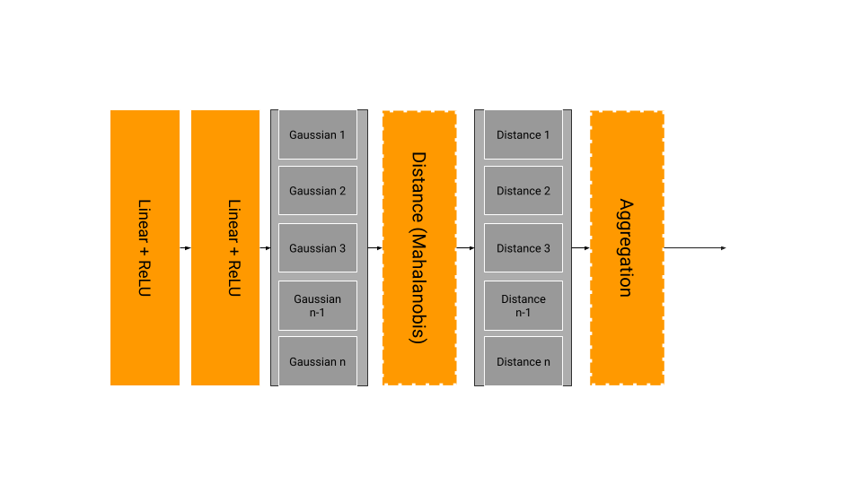
The diagram above illustrates the simple implementation of the model. When evaluated and compared with the existing baseline (v4 of AXOL1TL) over a number of Monte Carlo signals that simulate possible exotic signatures, we see an overall improvement, hinting strongly towards the success of the model.
| Process | Ours | V4 |
|---|---|---|
| GluGluHToBB_M-125 | 83.27 | 31.76 |
| GluGluHToGG_M-125 | 8.76 | 4.01 |
| GluGluHToGG_M-90 | 3.89 | 2.98 |
| GluGluHToTauTau | 3.23 | 1.99 |
| GluGluHTo2B2WtoLNu2Q | 41.26 | 26.64 |
| HHToBB | 80.01 | 58.04 |
| HHHTo4B2Tau | 74.97 | 55.97 |
| VBFHToTauTau | 12.27 | 11.84 |
| VBFHTo2B | 20.96 | 13.81 |
| WToTauTo3Mu | 0.12 | 0.11 |
| ttHto2B | 81.47 | 65.25 |
| ttHto2C | 83.70 | 67.83 |
The efficiency table above shows the efficiency of detecting the Monte Carlo signal when the trigger is operated at a working frequency of 1kHz.
VAEs with VICReg
We again go back to our discussion on VAEs, as the above method, though interpretable and better performing than the baseline (AXOL1TL v4), has a few shortcomings:
- Mahalanobis Distance for Gaussian Mixtures: The use of GMMs along with the Mahalanobis distance is not well defined when it comes to defining a single composite score/distance/metric. The said approach of using an aggregation function cannot be analytically justified and may lead to unexpected results.
- Computational Bottlenecks: The best-performing aggregation method for this use case is the geometric mean. We arrived at this result after extensive experimentation with various aggregation methods, including arithmetic mean, thresholding, and taking the minimum or maximum, among othersc. Implementing the geometric mean is extremely expensive on FPGA boards, making this model effective in theory but challenging to deploy in production.
The question now is whether one can design an estimator (of the MLP type) that can perform GMM clustering and subsequent distance estimation. Given that we are estimating the distance from the highly populated cluster, we can say that a VAE, when trained on these embeddings, can learn to reconstruct these strong cluster centres with more ease compared to the weaker anomalous ones. This is very different from using a VAE directly on top of the data, which can be better understood by revisiting the toy cylinder problem. The initial distribution of the data on the cylinder, though taken uniformly (for our ease), can be thought of as a combination of clusters. When density estimation using VAEs is performed on the input space alone, there is a strong likelihood that the model learns the entire distribution, as anomalies are not well separated in the input space. Moreover, due to the high dimensionality, the input space has a wider and more uniform distribution compared to the latent space, where the distribution collapses into clusters since the invariance conditions are enforced using the VICReg loss. The uniform/well-spread distribution on the input space makes it easier for the VAE to learn the entire input space, defeating our intention for it to only learn the statistically significant regions. When trained on the embedding space,, the VAE has a hard time learning to reconstructreconstruct small anomalous regions that are separated from the area of normals and are significantly outnumbered. The plot on the left shows our original input dataset, and the one on the right shows the nature of the embedding space.
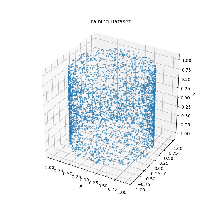
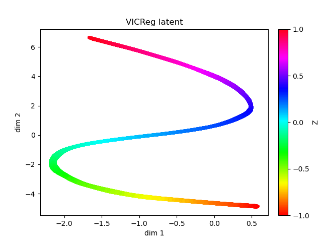
The distribution on the left (input space) is therefore easier for the VAE to generalize than the one on the right (embedding space). We can enforce this idea further by training a shallow VAE for the density estimation since embeddings derived from VICReg are disentangled, simplified and smaller in dimensionality making a shallow VAE sufficient to learn the normals Moreover using this setup we also successfully managed to incorporate some degree of physics information (that we can control through the augmentation) and detector information into the system by forcing the invariance. This lets us take the next step, where we add a VAE on top of the VICReg embedding. We follow the given recipe:
- Train VICReg with a suitable encoder on the raw data using physics-inspired and context-motivated augmentations.
- Strip away the encoder of the VICReg and freeze the weights.
- Extract the embeddings of the VICReg space.
- Train a simple VAE on the embedding space.
- Remove the variational part of the VAE along with the resampling step and convert it to an AE.
- Use the reconstruction loss between the input to the VAE (now AE) and output as the anomaly score.
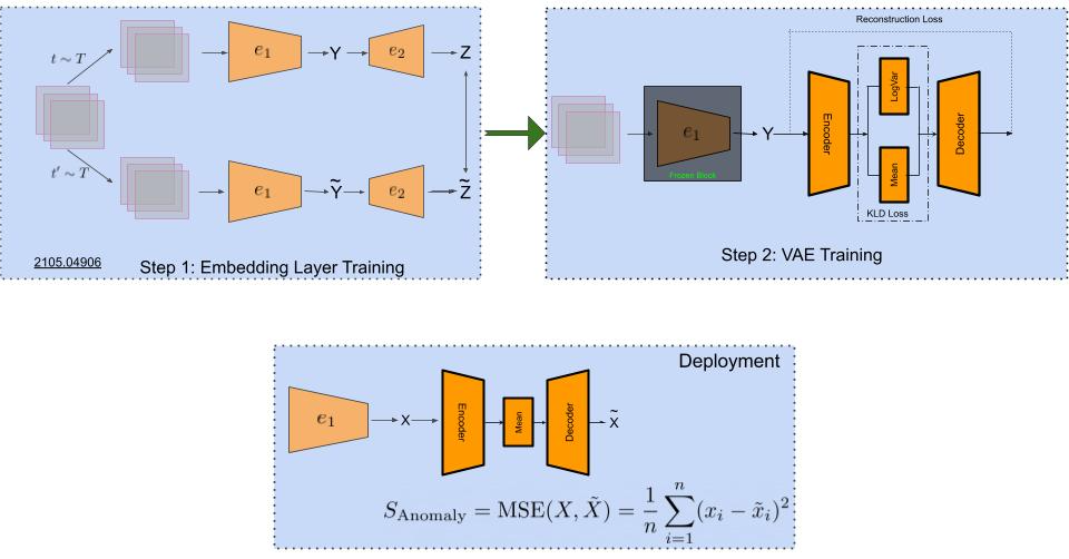
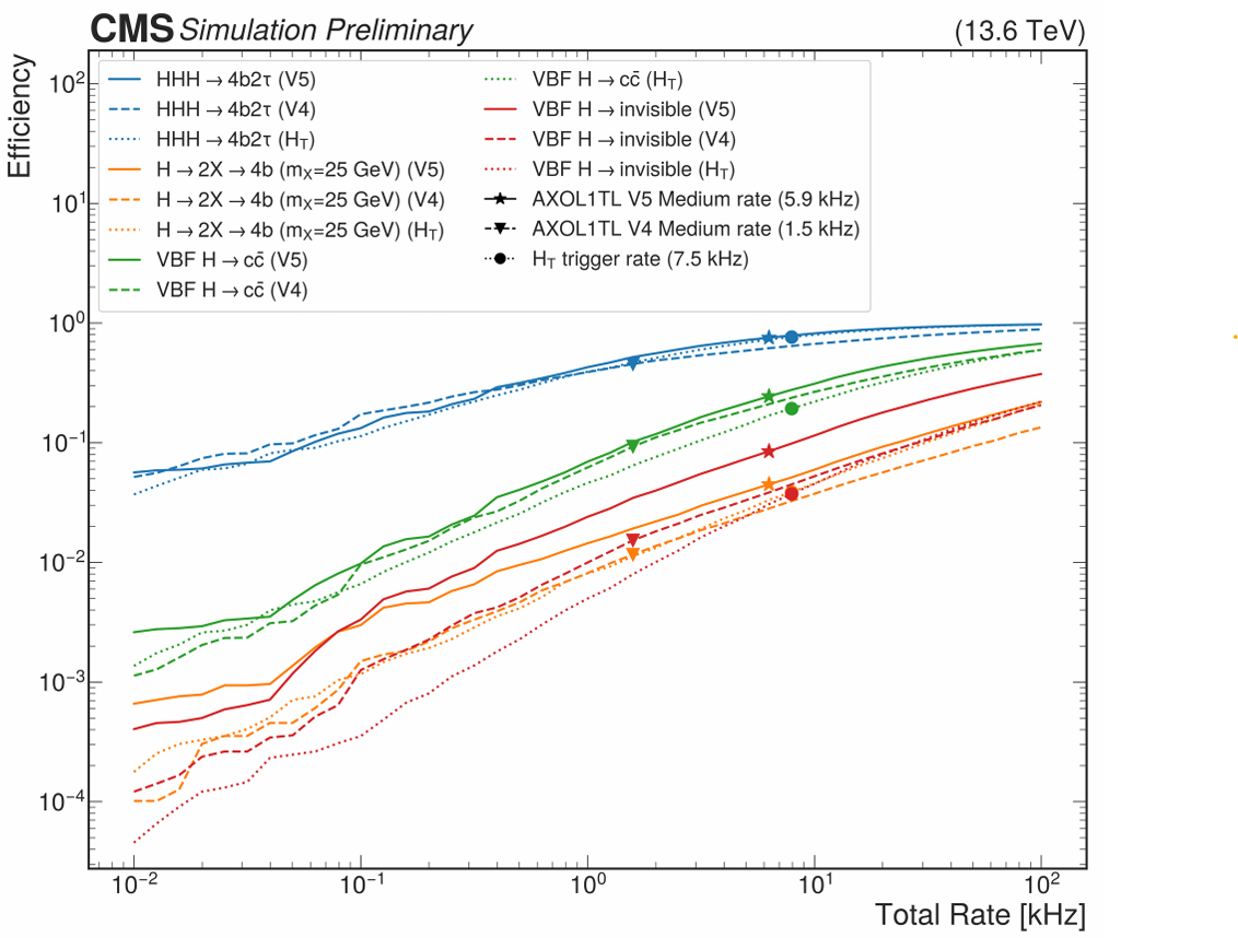
The above setup makes it very easy to deploy the above model onto the FPGA board, given that it is a stack of MLPs. Moreover, it outperforms the GMM+VICReg setup since the VAE backbox now manages everything. The comparison of efficiency in detecting exotic Monte-Carlo signals with respect to the last deployment (vanilla v4) is shown below.
The efficiency numbers for the V5 (ours) and V4 (old baseline) are as follows
| Signal Name | VICReg + GMM (ours) | V4 (Baseline) | VICReg + VAE(ours, deployed) |
|---|---|---|---|
| GluGluHToBB_M-125 | 83.27 | 31.76 | 95.93771 |
| GluGluHToGG_M-125 | 8.76 | 4.01 | 37.77188 |
| GluGluHToGG_M-90 | 3.89 | 2.98 | 15.854626 |
| GluGluHToTauTau | 3.23 | 1.99 | 4.831854 |
| GluGluHTo2B2WtoLNu2Q | 41.26 | 26.64 | 53.692781 |
| HHToBB | 80.01 | 58.04 | 84.302641 |
| HHHTo4B2Tau | 74.97 | 55.97 | 81.811932 |
| VBFHToTauTau | 12.27 | 11.84 | 26.036048 |
| VBFHTo2B | 20.96 | 13.81 | 27.53418 |
| WToTauTo3Mu | 0.12 | 0.11 | 0.270025 |
| ttHto2B | 81.47 | 65.25 | 86.183296 |
| ttHto2C | 83.7 | 67.83 | 88.221684 |
The efficiency vs Rate plot is given below. For the same budget (trigger rate independent of other triggers), both the v4 and v5 can be compared using the efficiency at the AXOL1TL medium rate.
For more details on the Model Architecture and performance, see